General stuff

At my student job,

• I started with porting a neural net script that was a part of a Research Paper, implemented in Caffe library to TensorFlow. Things were pretty straight forward, I had to get TensorFlow equivalent of the Caffe's weights.
• Construct the architecture defined in the paper in tf, load the weights. Here is when I explored sessions in TensorFlow, that lets me save weight loaded variables, that I can re-use for determining final predictions.
• This was followed by a bit of Image Processing where I had to segment the image semantically, followed basic approaches for the same. Have used the nearest neighbour to evaluate the semantic meaning of the pixels.
• Post this I had to explore techniques for anomaly detection - some of them were OneClassSVM, Feed inp to ResNet - use its features(last but 1 layer's op) as inp to the OneClassSVM, as I mentioned in the previous posts. 
• As of now working on trying to reduce the representation of a given image/patch (dimensionality reduction - basically projection the given data into a lower space) and then reconstructing the image/patch in that lower space. Post this, compute the reconstruction error to try and pinpoint the image/patch that was relatively difficult for reconstruction.

Anyways, now I want to explore semi-structured analysis (textual stuff), after a bit of exposure to a few NLP techniques at Uni, I am exploring the same a bit more.

I am not sure if I'll work on this, but I have an idea that I'd want to implement.

Recently, I got a chance to explore OCR a bit using this lib tesseract (https://github.com/tesseract-ocr/tesseract) - that is used for extracting text from Images.., and sometime later in a video on youtube, I came across this GloVe - Global Vectors for word representation, (https://nlp.stanford.edu/projects/glove/) which is a research by Stanford.

- So a text can be stored in several ways for performing analysis. 

- One way is to record each word's frequency and use Bag Of Words - vector representing the count of each word and its position.

- Or I can just use an incidence/boolean matrix, to just indicate if the word is present or not.

- But GloVe, it represents each word in a pretty epic way, by retaining the contextual meaning of each word. Each word is represented as a vector of several dimensions, such that, similar words have similar vectors (cosine sim might be high). 

So of course, there is a lot more that I need to explore about GloVe and its usage.

But I thought if I can combine OCR, use GloVe for the extracted text embeddings, and be able to summarize/ predict/ analyse the given text (preferably using RNN or something similar as it keeps track of the timesteps)(Not sure about this part, but I think as of now, I would consider it progress if I can do the OCR part + word embeddings using GloVe part)

Takeaways:

• Some insights about my part-time work.
• Initiate new exploration :) 

Uni Learnings

So, I thought I'll dedicate a post for the stuff that I get to explore here at the University. Also, include the topic/tasks that I am exploring at work - to have an idea about how the topics get translated to real-world use cases.

SVD - Singular Value Decomposition -

• From what I have understood, this lets me decompose the rectangular matrix into 3 parts - left and right orthogonal matrices and a diagonal matrix. 
• A use case for this was, in the Information Retrieval area, where I had like a sparse matrix - terms Vs document ..so like each document was represented by a  vector of 1s and 0s, where a 1 implied the term is present in the document, 0 otherwise.
• I can give this matrix to the SVD function, that spits out 3 very VERY useful matrices- 
• terms Vs topics
• topics Vs topics
• topics Vs documents
• So the topics are like categories to which the text belongs to, (Sports, Food etc),
• By mapping each of those terms to a set of categories and in turn using those categories to decide like the genre of the document is pretty cool.
• This can help me in retrieving documents better for a given query - by considering the context. There are ready-made functions for performing SVD, just have to str the data properly to feed it in.
• This is pretty cool especially if one is building some in-house information retrieval system for an organisation.

Map Reduce paradigm - 

• Framework for distributed data processing. 
• Damn cool technique iff, I can frame my problem as an MR task.
• In simple terms, there is a Mapper - (Sort and Shuffle) - and Reducer nodes that do-
• Mapper - Emits out Data tuples grouped by a key.
• Reducer - Gets the Key grouped list of data tuples and performs some kind of aggregation. (count, sum, max, avg...)
• One use case that I can think of is, lets say if I have several 1000s of docs spread across nodes in a network and I want to bring all the docs of each class in separate nodes, count # of docs in each class, perform some kind of textual analysis (relevance/priority), the Map task can like emit (category_id, <docId, content> ) and reducer will receive a list of (category_id, [<docId, content>,<docId, content>,<>....]) that can then aggregate all the tuples in the above list that belongs to a given category.
• Internally the framework supports the part where all similar docs are directed to 1 reducer only and also sorted. Uses hashing principle, something like, a doc that belongs to a category id '54' may be mapped to a reducer number given by 54 % #reducers (Ensuring all docs of category 54 will reside in the same reducer.
• There are several such intricate details in the MR framework and of course, Hadoop was the main framework that supported this I just need to write codes for the Mapper and Reducer task and rest everything is taken care. This can be used if 1 is searching for distributed processing (Of Course there are others like Apache Spark)

Signal Processing from IMU:

• If one is interested in making sense of the motion that is captured by devices like an IMU (that is built-in on phones), one can make use of this app called Science Journal by Google.
• That is a brilliant app that lets you capture acceleration (any axis), Ambient light in the room, sound, music and many more. It leverages on the IMU unit on the phone and lets u record stuff at will.
• The best part, you can download the captured information as a CSV!, and now it's just any other data.
• One can play with this data in several ways - 
• Apply a version of clustering technique (K -Means, Hierarchical, DBSCAN...) to the data to "discover" similar segments in the signal.
• With the knowledge of the type of motion, use this data to capture similar motions in the future, like a familiar gesture or something.
• Detect the amount of light in the room and act accordingly.
• Detect the level of the sound signal in the room and act accordingly.
• One can choose to integrate all this to like an app that he/she is developing.
• ML is just 1 step in the bigger project that can be developed.
• Or 1 can go all out, and combine all types of signals and determine activity.
• I can use the evaluation technique like constructing a confusion matrix (that captures False Positives, False Negatives and in turn Precision and Recall)

PCA:

• Very similar to SVD, this technique is done for Square matrices that capture data records Vs Features.
• If there are like 1000s of features in the given data and I do not know what to consider to perform analysis, predictions - I can rely on this technique Principal Component Analysis.
• That allows me to strip off some columns that are not that representative of my data in-comparison to other stronger ones.
• I need to construct a matrix called the correlation matrix that captures how 2 columns/features are correlated (as in, if an increase in 1 leads to an increase in another)
• Now, I need to perform Eigen Decomposition on this Correlation matrix, that spits out 2 parts-
• Eigenvalues and Eigenvectors (these are called the principal components)

• This works based on the rule, AV = ΛV; A- co-occurrence matrix, Λ - Diagonal Matrix of eigenvalues; V: Matrix of Eigenvectors
• So the vectors are arranged such that, the starting vectors (that are associated with largest eigenvalues) has the largest variance, i.e explains the data to a large extent in-relative to the ones that come later.
• So we can restrict by stripping of vectors/components that are at the later stages, that is not representative of the data and retaining top-k vectors combined with their eigenvalues as our new data that has been reduced to a lower dimension.
• This technique has been used in several areas including Genetics (to find the relevant gene), Eigenfaces - to generalise a whole collection of Human faces to capture unseen faces.
• Can be used in several areas (including Images for learning their features- pixels.. )

MinHashing:

• A technique that can be used for comparing documents that are too large to compare their raw boolean vectors. (where each dimension corresponds to a term)
• To do a raw comparison, metrics like Jaccard Similarity, Jaccard distance, Euclidean, Manhattan, L1, L2 norm and many more can be used.
• Jaccard distance although is very handy is computationally expensive(See formula) to be performed for several large sets.
• MinHashing is a technique that hashes such large column vectors of documents to signatures with much fewer rows. The technique is pretty cool,
• https://www.youtube.com/watch?v=96WOGPUgMfw&t=1080s
• The gist is, it considers a permutation of rows(which are terms in docs) and captures the index(row # in that considered permutation) of 1st word that occurs in the document.
• In the final hash, Number of rows = number of considered permutations, and it has been proven that determining the probability that the hashes of 2 columns (or docs) is same as Jaccard similarity of the 2 docs.
• Overall, one can use this technique if he needs to find similarity of severely large boolean vectors by finding the MinHash signatures of the vectors and determining the fraction of them being equal.

TF * IDF:

• Really cool scoring model for documents.
• One can use this while building an in-house retrieval system, by ranking each doc based on their Tf*IDF score for each term of the input query.
• Eg: If am searching for "Places I can visit in India", all the documents in the database can be ranked based on a score that is calculated for each term of the query and returns the docs in the descending order.
• TF - Term Frequency, IDF - Inverse document Frequency - Intuition is like, if the count of a term is too high in a document (term freq), that does not mean its important for that document, it also matters in how many documents the term appears (document freq).
• There are other complicated scoring models like the Okapi BM25...

Evaluation techniques:

• I can evaluate my prediction system, information retrieval system etc... using several metrics.
• I need to have the overall collection of docs at my disposal, which is relevant, irrelevant for a given query..
• I can use Precision that captures the fraction of the retrieved documents that is relevant.
• Recall - that captures the fraction of relevant documents that are retrieved, this is harder, as I need to know all possibly relevant documents for a given query, not just the ones that are retrieved by the system.
• F-Measure, the measure that is unbiased between precision and recall.
• I can use a matrix called the confusion matrix, that captures how accurate my model is.
• One needs to strike a balance between Precision and Recall, as too high Precision might come at the cost of a lower recall and vice versa.
• Precision, Recall and hence the confusion matrix needs to know the True Positives, True Negatives, FPs and FNs for determining the metrics.

The similarity between vectors:

• One can use Cosine similarity between vectors - that forms the basis for User-based and Item-based recommendation systems.

and many more..

Takeaways:

• Some of the good to know widely used techniques to get better clarity as to how one can go about processing the data at his/her disposal.

It has been quite difficult to keep up with posts. But it shouldn't matter as I am doing this as a release valve to sort of journal my thoughts.

So here is what I got to explore with respect to the CNN part using Neural Nets.

Having a basic, decent background in Convolutions/ Image processing from Uni, I referred https://www.datacamp.com/community/tutorials/cnn-tensorflow-python.

Tensorflow:

So from recent podcasts and videos I realised Tensorflow has this static way of creating Neural Nets, where I create a computational graph - basically I define a set of nodes in a graph that depicts the operations (convolutions/add/matrix multiply,etc..) for the incoming data, the edges representing the flow of data. (Although I came across Tensorflow 2.0 where there is an eager execution that gives one a lot more control to intercept data flow in the NN). Once I define the network entirely, I make use of the TensorFlow sessions to feed data into the defined the network. It Seems, this approach helps a lot to distribute the training process.

But it was a lot to code stuff from scratch, hence had to refer that blog, where I had ready-made code. I just had to understand stuff, which was decently hard, given the previous knowledge on Image processing and CNNs. But it was hard and confusing to run it directly.

Data Cleaning:

Had to realise this the hard way.
--
I got a chance to explore this technique called One-Class SVM for like a binary classification at my student job. Again, this was for Image anomaly detection. Overall, the task was pretty interesting, explored various approaches that I could have potentially taken. Some of them were:

- Give Image train data to the OneClassSVM API of sklearn, although it was a bit restrictive and not available in all versions.

- Apply PCA to the image data to retain the features/pixel data that explained maximum variance (shall try and cover such handy concepts that revolve around data processing/ pre-processing in the next post)

- Use ResNet to get The Most relevant features from the image and then apply PCA - post which gives the features to One-Class SVM. this was pretty interesting as per the link https://hackernoon.com/one-class-classification-for-images-with-deep-features-be890c43455d

- Lastly, it was the Autoencoder approach, which I have never explored, but I'd want to someday on an application that interests me. (semi-structured data)

But the sad part was, I NEVER really cared about how my data looked. I was in such a hurry to get the insights, I never gave a damn about the data. Unfortunately, it was largely crappy. It was skewed, un-curated, not representative enough, so I was asked to drop the whole task itself :( (time constraints)

--

Anyways, continuing with my exploration,

when I was about to drop the idea of using Tensorflow for this (which was pretty confusing for me - but was worth the experience), a friend asked me to explore Keras. It is too damn readable. 

A highly simplified way to define the network. This is when I realised, I NEED to stick to the larger picture in mind, no point taking a difficult path when either way I reach the same destination.

Currently exploring this: https://keras.io/getting-started/sequential-model-guide/

Built a basic NN using Keras with:

-32, 3 x 3 filters in the first layer (that took 1 channel from the inp image - grayscale)

-64, 3 x 3 filters in the second layer (depth 32 from prev layer)

-128, 3 x 3 filter in the 3rd layer (depth 64 from the previous layer - here, I realised, as u go further in the feed-forward network, the depth of the cube- Conv layer, increases rapidly, leading to HUUUGe number of neurons, in turn weights that is to be computed!)

-Flattened the layer (with prev depth 128!)

-A Fully Connected Dense layer with 256 neurons

- Finally a fully connected layer with the number of neurons that represents the number of classes that I want (in my case, the number of fruits)

- Forgot to mention about adding a MaxPool layer between each Conv layer, that halved the dimension, but retaining only the "strongest feature in the previous Conv layer".

- So, here each filter corresponded to an activation plane, that slides across the image, to "filter" out the "relevant" parts from the image. In other words, relevant neurons in the activation plane of each plane trigger the neurons in the next layer.

A few key observations:.

- Used Relu as activation for each neuron, that strips off negative values and retains max values. (there is also Leaky Relu)

- Use softmax (that gives the probability of each class) as the activation function of the last layer, that can be used to determine how relevant each category is for the Inp Image.

- Use batch gradient descent, that speeds up the convergence.(reaching the bottom of the loss bowl)

- Use Dropouts, that randomly switches off some nodes to increase the relevance of the final result.

- Use Momentum (that considers previous cumulative gradients- velocity+friction of the ball in the bowl, and current gradient - acceleration of the ball in bowl =- Andrew NG example) /Adam optimizer/ RMSProp optimizer.. and many more that can optimize the cost function.

- Like my Prof taught in class, Any model can be ultimately written as : 

hypothesis = regularizer + (regularisation constant) * (loss)

we just need to optimize the objective function such that the loss is minimised through (to find the weights and biases)
 Backpropagation - partial derivatives, Lagrange's Multipliers - KKT that can find the best values for weights across layers that minimizes the cost function.

- Use softmax - cross-entropy loss if using categorical values for the loss function,

- Can use Root mean squared error, mean squared error, L1 norm, L2 norm, Manhattan etc as loss function...or others if using regression ie predicting values but not categories. A lot to explore here.

But unfortunately, my PC is running out of juice, not able to keep the notebooks active. But as of now, I am getting a decent accuracy of around 73%. I'll probably either integrate this with the OpenCV that I had explored in the beginning OR explore something else.

Takeaways:

• Explore a lot more approaches/topics before sticking to one. As immediately boiling down to a selection can restrict the exploration stage.
• Its good to stray away from the main goal - Iff you can afford to do so - on the way u may stumble upon many more exciting things.
• Realised Videos/Podcasts/Tech talks, gives u whole new perspective towards things.
• Came across some really cool channels on youtube Lex Fridman, Strange Loop - this gives a good perspective towards translating ML stuff to industries. (Netflix one was really cool)
• The wave of examinations over the past months provoked me to at least document the topics that I came across while studying. Some of the techniques, tools are really handy and seems like it can be appreciated more if I have documented some of them here.
• As a next step, I'll try running the model against new images of fruits, see if it works, post that, try and see if it works for a live image captured from web camera.
• Also want to sort of exploring semi-structured analysis for textual stuff, NLP, TF * IDF, lang models etc.

It has been a pretty hectic semester. Hence not able to keep up with the writing. There are  lectures, assignments, student job.. lots to keep me active round the clock.

But the good news is that my lecture contents, and to some extent my student job as well, are sort of in sync with what I wanted to do here.They helped a lot to get a clearer understanding on certain topics. And also there is an exam on the topic in 2 days :D

So far, I've got a decent picture about Convolutions and incorporation of convolutions in the Neural Network with intermediate blocks Relu (to bring in Non-linearity), Max-Pooling, strides.. There is this awesome formula that gives me the dimensions of the filter outputs : output width:
 (initial width  + 2 * padding - Filter width) / (stride ) + 1

To sort of brief it up, here is what I could come up with, acc to my understanding:




So the story goes:
> I have the image of a fruit bowl and say I have a torch (with like a rectangular bulb to represent the square filter (5 x 5 x 3) as shown in the above image)
> I just slide the torch across the image - Each time when I am in a new position, I convolve(dot product) the torch with the corresponding area in the fruit bowl image where the torch is shining its light.
> The convolution operation is just multiplying the weights on the torch head with the corresponding image pixels in the area where the torch is shining its light.
> In the example picture above, the torch head is the 5 x 5 x 3 filter, and the area where the light shines in the image is the small red box , now I convolve these 2 to get 1 value which I store as a red blob in that second plane as drawn in the figure.
> Now I move/ slide the torch head - now the light is shining on the purple box. I convolve these 2 to get 1 value - represented as the purple blob in the second plane.
> Now I continue this and fill up that plane - this is called the activation plane.
> Activation plane represents the result of sliding the torch head (filter) across the image.
> Intuitively the filter tries to "filter" stuff out. As in, it could be a filter for detecting say edges or curves.
> Eg filter will have like

 to sort of detect the symbol 'U' and discard everything.
> So the 4 x 4 image regions having 'U' in them will have higher result in the activation map's neuron in relation with other 4 x 4 regions.
> Like so there could be several filters in 1 Convolution layer itself, which in turn results in that many activation maps.
> One can visualize this output of multiple filter as a box (number of neurons drawn are not exact):


So here, there are 4 planes in the box => 4 activation maps => outputs of 4 filters that were convolved with the input image.


> Why is this done?
> So that I can detect for eg blobs or polygons..shapes.. solid shapes etc in the next layer.
> Here the intuition can be a real human eye which detects stuff layer by layer:
     to identify an object, our brain first sees the edges(layer 1) then shape(layer 2) then the texture (layer3), finally recognize the object.
> The above box is essentially one more image/input with dimensions 6 x 6 x 4 .. just like the input image..
> Hence I can have additional filters in the next layers, by taking this box as my input and try run my torch against this new box.
> This leads me to being able to detect higher level features like say solid shapes...
ultimately the CNN structure might look something like :

((Layer - Relu) * m -  Max-Pool) * n - (Fully Connected Layer - ReLu) * o - SoftMax. (flicked from my lecture notes :D )

> Here, Fully connected layer is like the normal NN, where all the 35 * 35 * 3 pixels of my input fruit bowl are connected to specified number of neurons. This is super complex operation, hence not used since the beginning of the layers... Hence the torch sliding helps reduce the number of computations.

So the ReLu, Max-Pool, SoftMax are pretty intuitive concepts which I shall be covering in the next post.

TakeAway:
> Bigger picture of what CNN is all about how one can detect stuff with a CNN architecture.
> Bit deeper into the workings.
> Intuition on Convolving a filter across an image.
> Concept of filters.
> Interpretation of Filter outputs as neuron-contained activation maps.
> On a side note, I might consider using tensorflow for directly building a basic CNN and train the model. Not sure when, probably after exams.

Begin.

It's been a while, caught up with exams, onset of overwhelming yet exciting subjects of the new semester.

So a couple things happened actually,

> Started exploring the implementation of basic neural network on the web. (without the optimization or even the validation part!). Main intention was to see the entire flow in action hopefully in a graph!).
> After some googling (there were ready codes available):

Here is what I tried to implement -

> I decided on a basic neural net structure, straying a bit away from what I wanted to be able to predict in the first place.

> This is what I wanted to implement

A few things that I explored on the way-

> I used a dataset that was given as a part of a course by my Uni, (Titanic survival dataset- which I think is available on Kaggle).
> I wanted to play with the dataset, hence explored a bit of Pandas - yet again, it is one powerful and beautiful utility! Using jupyter notebook as its just awesome.
> Realised Pandas understands data in terms of dataframes, awesome way for filtering, doing a basic EDA on the given data to get like an overview of the data.

> 1 important step which I had to unfortunately realise the hard way, was the part where I had to thoroughly 'clean' my data.
> Here, I explored why I was supposed to clean the data / How can i do all this in Python
              1. Remove NaN - non numeric values.
              2. Convert categorical data to numbers (Enumerations)
              3. The important one was Normalisation  - Sort of having all of the features in a standard scale. Like there could be a column A whose range is 1-5 and 1 more B whose range is 1000-60000. > So in this case, if they are used the same way, as pointed by this person on youtube, the weights assigned to those features might heavily rely on the numeric values alone and not its influence on the result - as in, if A has the value 5, B has 1000, B might be given the wrong weightage.
              4. Hence normalize using, X = (val - mean) / standard deviation - Stand deviation describes the spreadness of my column.
              5. To sort of squish the values of a column btw 0 and 1, I can use X = (val - min)/ (max  - min)
              6. Initialise the bias column (np.ones) to X.

> So I wanted to predict the age of the passenger given his/her features - something like, given his/her economic status(class), location....accompanied by .. price of ticket purchased... , try and guess their age.
After cleaning the data bit,  I decided on the label (age)..

> O, I also need to squish the Y or labels between 0 and 1! as my NN gives me values between 0 and 1! Totally forgot to do this till the very end, hence I used to get faulty error function! Error function had errors :D


> Formed the backbone of the NN that had like 2 internal layers excluding the input and output layers.
> The weights to a layer followed the format:
ex on layer 1
[
     [weight on neuron 1, weight on neuron2, weight on neuron 3 ],  // for feature1
     [weight on neuron 1, weight on neuron2, weight on neuron 3],  // for feature2
     [weight on neuron 1, weight on neuron2, weight on neuron 3]   //for feature3
     [0.1, 0.1, 0.1] //bias weights
]

> I had to initialise the weight matrices (numpy.random.rand) - initialise bias weights (0.1) as well.

> Multiplication between several matrices was a pain! was too hard to ensure the shapes of the matrices are to be maintained - obviously I could not figure stuff out myself, went wrong at several places real badly, hence I referred the web.

So the structure was something like:

> Also yes, for backward prop (climbing down the error hill), the gradients for all 3 weight matrices for 3 layers, unfortunately  I referred the web for the ready made formula - but yes I understood the partial derivative part and how they derived the gradient wrt diff weight matrices using chain rule.

So this is the cost function (difference between actual and predicted values) that I plotted using Matplotlib



So yea, the flow seems okay, as in -
> Yes the cost function seems to be decreasing. So the offset btw the actual and predicted values seems to be decreasing at every run.
> But 1 main thing that I am not doing here is the validation and optimization part..
> This expects me to address train - cross validate (model evaluation) - test (error) part.
> And also if there is overfitting or underfitting in the model. Apparently there are techniques to prevent model from overfitting (the selected weights for features is highly inclined towards the training set and does not generalise well for new incoming data)
or
underfitting (the selected weights for features is highly generic and does not predict stuff well)

> Some of them are -
                   Have more data,
                   Regularization,
                   Drop Outs to prevent Overfitting.
                   Change network architecture
> Techniques to rectify underfitting  -
                   Have more layers
                   More neurons in each layer
                   Change net architecture

TakeAways:

> Need to decide on the neural net architecture first -  layers, neurons, learning rate, num_iterations and stuff.
> Data cleaning - data munging - data wrangling - to clean non-numeric values, enumerate categories, normalize the data(features and labels).
> Initialise weight matrices - add initial bias weights column (column of some 0.1 initially) as well!
> Add bias column (column of 1s) to the input features. (bias - used to fit the model better)
> Pandas for data exploration - dataframes, effective filtering, selection and manipulation of the data.
> Understand how the feature matrices are represented which when combined with the weight matrices results in activations that is passed onto the next layer.
> Ensure the shapes of matrices are maintained across layers.
> Understand how gradients for different weights are calculated using back prop and hence the partial derivatives (chain rule was confusing!)
> The chain rule formulas are faulty - as in
             - the biases that were added in the beginning to the features and weight matrices had to be handled for each weights.
             - had to transpose a couple results to ensure right shape is maintained. Was confusing! Hence copied off the formulas from the web.
> Satisfactory decrease in the cost function across iterations! Plot was nice to visualize:) but unfortunately have handled nothing.


> Need to incorporate train_cross-validate_test split for validation of the model.
> Also need to incorporate regularization, drop out to prevent overfitting(inclined to train data)
> Explore possibilities of underfitting as well.
> There is also something called gradient checking to double check if the gradient descent achieved in the model was right.


> Offf, that was a lot I had to explore in parallel with other things, I think some of them were incomplete...but its fine..I think I have a fair idea about the story..,
> for the next steps, with this background , I think I'll dive into CNN, and learn on the go types  (Optimizations can be done directly wrt CNN)
> Have also enrolled for Coursera's Andrew NG's Deep Learning course. (One can audit this as well for free!)
> Have also audited the course on linear algebra on Coursera - the math for ML.. to sort of be able to appreciate the math better! Not sure if I can keep up.

Also, not sure if posting the code makes sense. I feel the satisfaction to see one's own code in action is awesome! So, even if a bit of effort is made to go out there, make an attempt to understand already written code snippets (which they say is far more challenging than writing ur own code), is worth it! :)

End.

CNN contd..

 Ok so far, I've understood -

> Forward propagation - where I calculate the outputs for a given layer using the outputs from the previous layer by fusing them with  previously initialised weight matrices.
> Gradient descent to calculate gradients that would be subtracted from the weights assigned to the neurons in order to minimize my error.
> The decrease in weights has to be done across ALL layers.

Consider the example:

The second layer weights has the shape (2,3) - to map 2 outputs of previous layer to 3 neurons.
Hence layer2's weights is given by a single matrix.

> layer 1's matrix : X = [x1 x2]... (1,2) shape

In reality X will be a 2D matrix, eg:
X =[
             [f1,f2,f3],   #row1 in our case, probably a row of pixel values of an image
             [f11,f22,f33] #row2
      ]

W1 = [
               [w11 w12 13],   # maps x1 to all 3 neurons
               [w21 w22 w23] # maps x2 to all 3 neurons
         ]... (2,3)
W2,W3.


similarly, for other weight matrices.

> So using the weight matrices in each layer, I calculate the activations of the next layer. (Matrix Ops)
> Next I need to calculate the final error J(W) = (actual value - observed value)/ total    #avg

> J(W) depends on the final weights W3 which in turn  depends on W2, that depends W1 which depends on the input features(X).., I think intuitively it makes sense as the next activations were calculated using previous weights to this layer and previous activations.

Now, I need to rectify my error a.k.a change my weights

> Backpropagation - So I am backtracking starting from the last layer towards the first layer to see how each of the weight matrices is having an influence on the final error.
> I also realised in the last post, in order to get how a variable independently influences a function, I need to consider all other variables as constant and take the derivative of that function w.r.t the variable of interest. This is sort of the definition of a partial derivative of a variable.
> So I take the partial derivatives of the final error function with respect to individual weight matrices and propagate that back to the respective layers so that they can "tweak" their weights accordingly.

Something of this sort:
J(W) = (blah)(y-y^)   #y - actual value

y^ = a(z(4)) #a-activation function
z(4) = a(3) * W(3) #W(3) is the weights used to reach layer 4  from layer 3

a(3) = act_function(z(3))
z(3) = a(2) * W(2)


a(2) = act_function(z(2))
z(2) = a(1) * w(1)

a(1) = act_function(z(1))
z(1) = X * w(1) # X- inp features


So I can say that -

changes in J w.r.t W2 =(change in J wrt y^)
                                    *(change in y^ w.r.t z(4))
                                    *(change in  z(4)  w.r.t a(3))
                                    *(change in a(3) w.r.t z(3))
                                    *(change in z(3) w.r.t W2)!!

Need to do this much which I then subtract from the existing W3. This is sort of equivalent to me "taking a step down" from that hill seen in previous posts (w.r.t W3!)..

> I have tried not to include any formula to sort of retain continuity, as formulas intimidate me! (although once I understood the story , it shouldn't be hard to understand them as well)

> With a decent background in derivatives, I could follow the backprop on the web with formulas.
(just skimmed through the one given in matrices.io website)

https://matrices.io/deep-neural-network-from-scratch/

> I just had to know the derivative of hyperbolic tanh as they have used this as activation
function(tanh)..

> Now that I know the story of  forward prop, backward prop - how backward prop uses partial derivatives to carry backward the error caused by the weights.

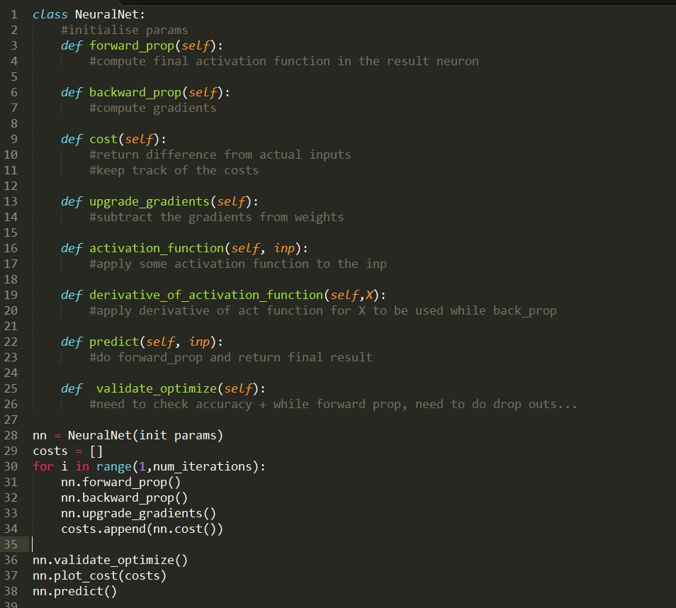
Pseudocode could be like:

for given number of iterations :
     forward_propagation( ) #predictes stuff
     backward_propogation( )  #calculates gradients of all layers in the backward direction
     update_gradients()

  > update the weight matrices (w = w - alpha * gradient_w).... alpha - learning rate
  > the shape of a weight matrix w and gradient_w has to be equal as it is element wise subtraction
  > the element wise subtraction implies how the weight of each feature is decreased accordingly - something like how important is a given feature on a neuron of a layer.
 



Bias:
> Had left this part for a while, as I thought it needed formulas for understanding bias.
> Now, the activation function that each layer determines, given by:
 a(layer) = activation_function (z(layer))
 where,
 z(layer) = a(layer -1 ) * weight(layer - 1) #FMI : a(0)  = feature set

> This activation is a nonlinear function that transforms the linear equation :  features * weights so that patterns can be found, various other non-observable patterns can be found, using which probabilities of getting a value can be determined that squashes the result between 0 and 1.

> Some of the functions that I came across were the tanh(hyperbolic tanh(x)), Relu (rectified linear unit), Sigmoid - apparently there are lots of them, which one to choose - not discussing that now - ill probably refer this when required - 

http://cs231n.github.io/neural-networks-1/     #refer commonly used activation functions.

> Now, on using a website https://desmos.com, I plotted the tanh function to see how it looks

a = tanh(x)
looks something like

   







Clearly the y values are between -1 and 1 and I see the graph ascends to 1 at around x = 0.5.

But what if I want the graph something like,

The above graph has the equation
a = tanh(x -1.4)


Where the graph has a sharp ascend at around x = 1.4 ... probably this predicts stuff better...

>Now that -1.4 is a variable and I do not know the "correct" value with which I can determine based on the training set. And I call this value the "bias" that helps me construct my model.
> Hence I put bias also as a part of the weight matrices which I will use in both forward and back propagation.
> The feature corresponding to bias will just be a row of 1s and corresponding row of 1s in the weight matrices.

>Now, because I am subtracting say a gradient w.r.t W3 from the actual matrix W3, it's obvious that both of their dimensions need to be the same.

eg : If a(3) has the shape (5,2) and a variable delta has the shape (5,1) and gradient_W3 = delta . a(3)
and the actual W3 has the shape (2,1) - I need to transpose the matrix a(3) to make it (2,5) so that
(2,5) . (5,1) = (2,1) which I can use for an element wise subtraction.

Handling bias in gradients..
>Bias - To cater to handling gradient of bias - in the eg:
 z(3) =  a(2) * w(2)
w(2) will have an additional row for bias, but its gone while z(3) is calculated, hence while calculating the error (backprop :  gradient_w2 from z3)  w3 is having an additional row for bias -  need to cater to that as well, hence the formula for back-prop takes care of that as well.
> But the additional column added to the gradient for w3 cannot be used for back propagating the error calculation for w2, it needs to be removed.
> If the above is too difficult to understand, I can just stick to that website, it mentioned a bit clearly.

PS:
The formulas to calculate the gradients in backpropagation,
adjusting the matrices of activations (transposing) to match the weight matrices,
adjusting matrices to include bias corrections and re-adjusting such that they are not propagated
is all compiled in that website.

It might get complicated, I believe the formulas can just be briefly seen, just need to get a vague idea about what is happening.. But it's a nice exercise for the brain to try and understand the formulas from that website .


TakeAways:
- Forward propagation - calculate activations in each layer using previous layers' activations - finally predict value
- Use the above to calculate error.
- Back propagation : Starting from the last nodes, calculate the gradient wrt the immediate previous weight matrices (partial derivative)  and use chain rule to propagate the error to previous layers (by taking partial derivatives  of various weights ).
- Can check desmos.com to realise why we need biases.
- Update weight matrices using the calculated gradients from the previous step (don't forget learning rate - that decrease the step size while descending the hill)
- Adjust the activation and biases while back propagation.
- General pseudo code is given.

- Finally I think I have the stuff to have an end to end crude NN setup (without any error handlings)
- Shall try and implement stuff in the next one! (for sure this time! :-| wanted to have this post as I had left out backprop and bias)


End.

CNN contd..

> Now, the graph that I had in the last post, did not explain everything in detail.

> It was a graph of error function J(W) (y-axis) vs 1 parameter (or 1 weight ) that is supposed to be multiplied with 1 feature.
> But in reality there are large number of weights (in matrix forms) that is multiplied with features.
> Implying the fact that, the error function or the cost function is affected by each and every weight parameter that is used across all layers of our network.
> So, now how will I get to know how my error function changes once I change my weights. Cannot really rely on a 2D graph..

> So, I need to be able to constantly change all of my weights such that the error decreases in every iteration.

> But by how much?

This is when I came across gradient descent, which says use a 'gradient' to change the weights that u initially used to predict the final class.

Something like :

for each iteration:
    for each layer i :
      gradient_w11 = determine_gradient_for_weight_on_neuron1()
      gradient_w12 = determine_gradient_for_weight_on_neuron2()
       ... and so on
   
      new_weights_on_neuron1  = original_weights_on_neuron1_changed_by(gradient_w11)
      new_weights_on_neuron1  = original_weights_on_neuron2_changed_by(gradient_w12)
      .. and so on

      calculate_error_with_new_weights() //check if this is decreasing!
     (in case I forget : error is the potato being predicted as a book!)
 
> Ofcourse, I won't be calculating the gradients for each weights on each neuron individually - as in its all using matrices! (Numpy)

>Now, how is the gradient computed:

>This is where the math that I was taught a couple years ago comes into the picture.
It's about finding the derivatives of  functions (differentiation). So the derivative of a graph a.k.a slope of the tangent to the graph - according to my understanding -  will give me the direction of rate of growth of the function.

> This is what I understood -  if any 1 comes up better/simpler understanding, pls feel free to post in the comments.

This is what I found on google images. Its actually from this youtube channel 3blue 1 brown. that is pretty amazing! (https://www.youtube.com/channel/UCYO_jab_esuFRV4b17AJtAw)

So bottom line, if we assume the graph on top LHS  as our error function (probably with 2 weights vs error), and take the derivative of the error function (with respect to weights), we get the direction of growth of the function..

But we want the exact opposite thing!
We want to descend that hill.
Hence they have told, reducing our weights by the obtained gradients, enables us to descend the hill on the left  => implying that we are trying to obtain the weights (for our features) for which our error (graph on left) is minimized.


I think intuitively, it makes sense, gradient tells me by how much the function grows wen I increase my weight. If I decrease the weight by that gradient, the function comes down right.

Now, the derivative that I talked about, can be with respect to any of the weights.
The derivative for the graph/error function (y = f(x) ) or dy/dx form - tells me how the function y (error) changes (more like increases) , when there is tiny change in the value of x (weight).

> On similar lines i'd want to know how the y function changes for tiny changes in weight w11,w12,w13,w14........ and so on..

> For this, there is this partial derivative, which says how the graph/error function/y changes for tiny changes of a particular variable (weight) while others (other weights) are treated as constants.

>Something like:

for a given number of iterations:
   for each layer i :
      gradient_w11 = dJ(W) / dw11   #error function J(W)
      gradient_w12 = d(W)/  dw12   #the symbol needs to be a lowercase delta not 'd'
     ...
      ...and so on for all the weights

> Again, in the above step, everything is done matrices (Enter NumPy!)

> Ok, now that I have my gradients, as I said above, I just need to subtract this from the original weights to descend down the hill (similar to sliding down the bowl!)...
i.e

original_w11 = original_w11 - gradient_w11
original_w12 = original_w12 - gradient_w12
... and so on (but using matrices in a single step!!)

> Now, consider this example,
#prediction function
z = 2(w_1)^2 + 4(w_2)^3

partial_der(z)/ w.r.t (w_1) = 2 * 2 * w_1 + 0        --- gradient_w1
partial_der(z)/ w.r.t (w_2) =  0 + 4 * 3 * (w_2)^2 --- gradient_w2

Now if my original weights for my features were , w_1 = 4; w_2 = 3

z = 32 + 27 * 4 = 140

//re-assigning my original weights

for w_1
w_1 = w_1 - gradient_w1
w_1 = 4 - (2 * 2 * 4)  = -12

and for w_2
w_2 = w_2- gradient_w2
w_2 = 3 - (4 * 3 * 3)^2  = -1293

now my new prediction z is
z = 2  * -12 * -12 + 4 * -1293 * -1293 * -1293!! that's a lot!
but the transition seems too damn high!! from 4,3 we reached -12,-1293 !! :-O

we might have actually missed the minimum value from the error function,
 something like

 So we might have jumped right across to the other side of the graph (of course the graph does not exactly correspond to the weights' example I've shown above)





So we need to jump down slowly!! In smaller steps!

So Now, there is this term called "learning rate" (alpha symbol)  that I can use to control my steps.






Something like:

w_1 = w_1 - (learning rate) * gradient_w1
w_2 = w_2  - (learning rate) * gradient_w2

Now, if I take my learning rate to be like 0.01 or something, and plug in the values in the above equations, I should get a decently small value resulting in

So that is good, and there is still hopes of reaching the bottom or minima or global minima where I can be assured that my system will accurately (to some extent!) predict that food item is a potato and not a book!

(FYI- the left image is again, only with respect to 1 weight!! so its weight vs error function)


So the challenge is to choose the best learning rate (alpha) so that the steps aren't too small  to an extent that the system might take ages to reach the minima, i.e they say the model will take a long time to converge!

We don't want that, or do we want the system to shoot up to the other side of the graph, clearly missing the minima just because we choose a large alpha (learning rate).





TakeAways:
> How gradient descent works - derivatives of a function gives the direction of rate of growth of a function and we want to go in the opposite direction.
> I achieve the above by taking partial derivatives of my cost function with respect to each of my weights on each neuron across all layers! Ofcourse, I need to do vectorised implementation of this. No loops!
> Ofcourse, I cannot be all greedy and decrease the weights left and right! This leads to me missing the minima (the point where the error is minimum) and jumping off to the other side of the bowl..
I need to carefully choose something called a learning rate that I will use along with my gradient while descending the hill. (while am subtracting the original weights)
> Some of the above facts might be redundant, but point was to emphasize on certain things, to make myself understand it better (even the pseudo code is for the same purpose)
> Hmm, I might have enough things to try out few things like say,
Initialize my :
 - input, output and hidden layers - number of neurons on each layer - Initialize weights for all neurons across all layers - choose a learning rate - number of iterations for my gradient descent (how my time do I take the steps down the hill)
- compute outputs for each neuron, across layers and finally predict the output.
- Not sure, If I can also implement gradient descent (back propagation - ofcourse I will have weights multiple layers which in turn makes the calculation of partial derivatives in each layer difficult ), as I still need to know what the partial derivative formula is (chain rule).

- Oh yea, I haven't discussed about the bias which I will be adding while multiplying the weights with features, I ll probably bring in some activation function as an example (tan h, relu, sigmoid) to sort of visit bias usage, also probably talk about whose partial derivatives I should be calculating - for which again I need to make use of an activation function.

- So as a part of the 'sub-idea' that I would want to work on, post covering the concepts of backprop and bias in NN, I would want to implement the entire flow, without any libraries - do not care about the accuracy, but I would like to see the cost being decreased at every iteration and weights getting updated, I ll obviously use stuff for references, but i'll try writing it myself.


End. 

CNN contd..
Begin.

> So, before I start understanding Conv Neural Net in more details, I thought ill explore a bit more of basic Neural Net.
> After a bit of googling and youtube, I came across this site that had 1 of the best comprehensive detailed description about Deep Neural Net.
> It is simply mind blowing as to how they could accommodate all the necessary information. They have everything - best part  - they have used an example to explain the flow.

https://www.matrices.io/deep-neural-network-from-scratch/

> Yes, it's a huge post, but I believe I can revisit this several times if needed, but the way they have described it is beautiful.
> From going through like half of the page contents - I am able to have a fair understanding on things like -
 - Represent features as matrices
 - Feed the features into the neural network
 - How the NN fuses the features with weights. Matrix multiplications of weights.
Something like:
for each layer:
   for each neuron in a given layer:
     for each given feature from previous layer:
       z = (feature) * weight on the neuron
       res = some_sort_of_non_linear_function(z) // so, some of the functions could be - ReLU, sigmoid, tanh... basically they squeeze the res btw a given set of ranges which can be used by us for setting a threshold or cut-off for predicting valid results.
____
> Now I cannot afford to have the above loop as it is computationally expensive for the computer.
> Hence the smart people have come up with vectorised computations (using libraries like numpy where they make use of optimized underlying C functions)

> A line in this below post said : ' the vectorized NumPy call wins out by a factor of about 70 times:'

https://realpython.com/numpy-array-programming/

Here, they try to calculate the maximum profit when u r asked to make 1 purchase and 1 sale. They have 2 versions of the same - loops and numpy -  Numpy seems super simplified (2 lines!).
____

So, continuing with NN,
-  The output is called the activation function (non linear function)
- Realised how output of 1 layer's neurons is passed onto the next layer.
- In general, when I talk about each layer, the task of multiplying previous layers' outputs (if previous layer is the first layer - then input is the given features) with weights of all the neurons of this layer can be expressed as 1 step!

Some videos that I saw:

https://www.youtube.com/watch?v=aircAruvnKk

https://www.youtube.com/watch?v=2-Ol7ZB0MmU&t=1062s

There are a lot more stuff that I can visit, understanding has been a cumulative process.

Little beastly matrices for math!


From that website (matrices.io),
> I could make sense of what I have written on the LHS, x1 and x2  are the features (in my case, pixel intensity of the food at top left and bottom right corner) in first layer
> There are 4 neurons on the second layer with their own weights expressed as a matrix.
> First row corresponds to the weights for the feature x1 and its connections with the 4 neurons in that layer.
> Same goes with the second row of the weight matrix which is wrt the second feature's weights for all 4 neurons of the second layer.
> On asking numpy to multiply this, we get a variable Z which we give it to the symbol σ which is the activation functions (ReLU, sigmoid, tanh...)

> Now we have values that we can probably use to predict the final class (food ingredient), but what about taking care of the correctness??





Error Optimization:

I cannot afford my system detecting the object to be a book when it's actually a potato (but what if its a book that has a potato pic.. hmm.. for next time)!  

> The website had summarized certain things I could actually relate, things like how I compute my error (predicted value - actual value) 
> its the J(W) formula that I have written above - they call it the cost function (that tells how much is the error) which we need to minimize.
> the formula is actually intuitive, y is the actual output class (potato), y^ (book) is the calculated value, have used squared function to remove negative, have summed things up to get like a final accumulated collective error.

> Now, that error function is a convex function that is of the form like y = x^2  like a bowl shaped graph, once again, indicating that it actually has a minimum value (bottom of the bowl).

> So this is my error function and am here right now,

But I want to reach here! Hence I badly want to slide down (gradient descent) this bowl to the bottom.

TakeAways:

> So bit more on how I can represent input features and   - weights on each neuron across layers w.r.t each input feature -  using matrices. (each row in weight matrix represents each feature's  connection with all the neurons in that layer)
> A rough algorithmic steps involved.
> Some sort of mathematical description (image)
> How numpy is all being boss when it comes to computations.
> Its a book! Not a potato?? No can do!  - this is where I cannot afford to overlook error optimization - which I realised is a bowl and I just need to slide to the bottom and it's all "downhill" from that point :D 

- In the next one I intend to write a bit more on gradient descent (which is the technique for sliding down the bowl) and back propagation which is the technique used by our NN to calculate errors.
- Post this, probably try and implement a basic "sub-idea" NN to see stuff in action.
- And yes, I havent mentioned about the 'bias' thing that I have written, shall visit that as well.
- Then visit Conv NN.
- Exams going on, might get delayed by a bit. End.

Convolutional Neural Network:

Ok so here is what I have understood so far. The story might be wrong, vague, in which case, do let me know.

> Of Course the way I have understood might need a lot of refinement, but this is based on what I have accumulated over the past 2 days through the web.
>I shall try and keep it as simple and intuitive as possible(say like if a person like myself doesn't have the necessary background).

> So for starters a Neural Network is a network of neurons spanned across multiple layers.
A neuron, just like a brain's neuron accepts several input signals (input features in our case) and spits out an output signal (output value).
> A simple neural network can have like

 

This is exactly what am trying to do but for identifying food ingredients.

> Every neuron accepts the features (in the above case - image pixels), multiplies those features with certain weights and passes the output to the next layer.

> The above steps are done in a very cool way using matrix operations using libraries like numpy in python as it is wayy too faster than having several loops.

> In the last layer (output), there are 2 neurons - each of which will have a probability value, that gives an information like - "how sure it thinks the picture is a cat or a dog"

> Now, this probability is what we are trying to optimize for correctness

.

> If we backtrack, the thing which is under our control is not the features, as that is our input and we cannot change that, but the weights - those weights were decided upon by our neural network.

> Hence, optimization of the neural network involves something called a backpropagation (gradient descent ) that "tweaks" or "tunes" its dials to "rectify" those weights to cater to identifying the cat or a dog picture correctly.

> So the network has to "learn" to do this. Hence it learns when we give it certain "correct" results. Hence this is some sort of supervised learning where we supervise or monitor if the learning is happening properly in contrast to unsupervised learning where the neural net thinks its smart enough to give accurate results without asking us for already correct results.

Relate:

Now, for my requirement, in the end -

- I would like the computer to "see" the food items and try and identify the food item correctly.

- Hence my video feed is the input to the neural net. Video is nothing but a stream of static images, hence image is my input.

- So if am able to do this first, when I throw an image at the neural net and it is able to identify the image, I think I might have gotten closer to the final result.

- But from what I know thru Open CV, image is a 2D array (not considering channels as of now). So there would be huge number of neurons if I were to represent each pixel as a neuron and it is way too costly.

- Hence the smart people have come up with something called Convolutional Neural Net where there is some sort of windowing is done, which I ll try and describe in the next post.

TakeAways:

- Neural Net has several layers of neurons.

- Neuron takes several input features and spits an output - Does this by multiplying input features with weights  - and subjecting the result to some sort of function (activation function) to spit out a value.

- Based on the output I try and predict the result, hence I need to optimize the weights.

- Optimization is done through back propagation - which involves determining the amount of error (that is the difference between the correct output and the predicted output) and "tweak" my input weights.

- But for an image, normal method of giving image pixels to neurons is costly, hence I refer to a convolutional neural net approach.

- I realised by taking a top down approach when we learn something, we appreciate things better. Yes I know we might not have an in depth understanding of the topics, but I think its okay, as eventually we will get there if we pursue it long enough. But initially, if we have some sort of motivation, real world use case, wen we explore something, we definitely will appreciate it better. (And this has to be the case wen one starts his bachelors course)